人工智能—Python實現線性回歸
1、概述
(1)人工智能學習
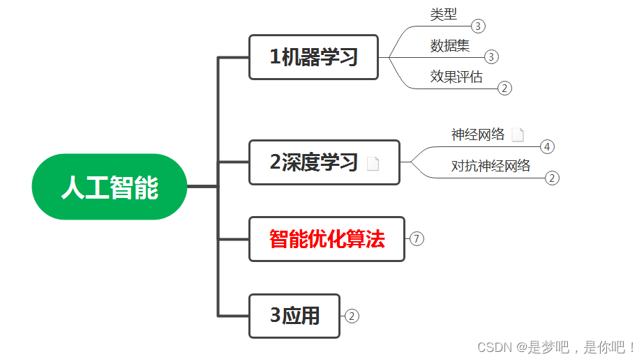
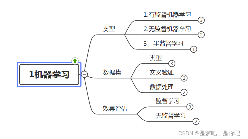
(2)機器學習
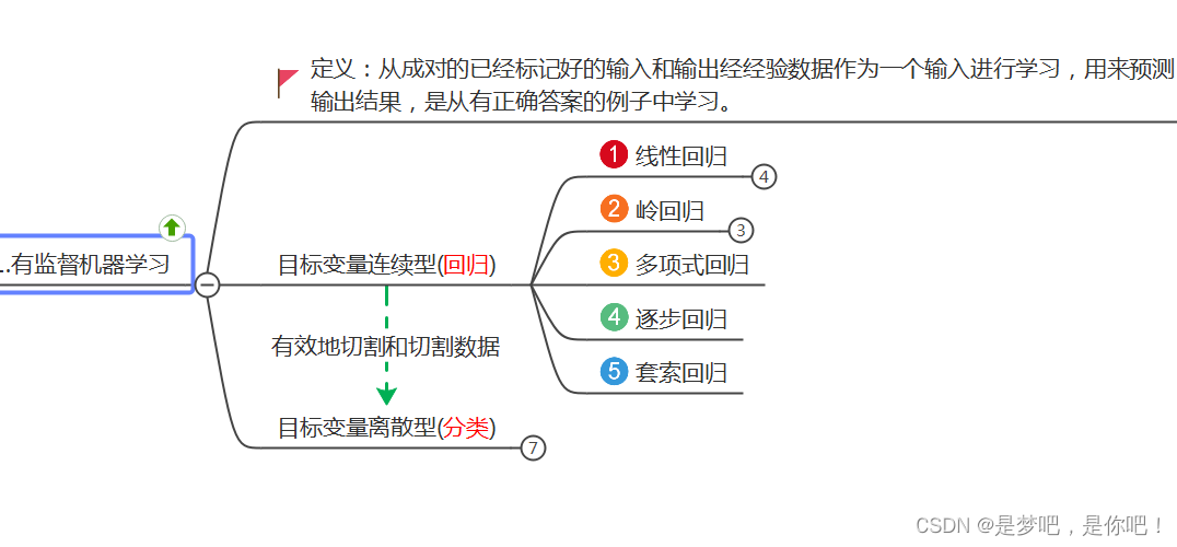
(3)有監督學習
(4)線性回歸
2、線性回歸
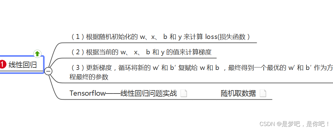
(1)實現步驟
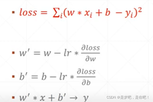
- 根據隨機初始化的 w x b 和 y 來計算 loss
- 根據當前的 w x b 和 y 的值來計算梯度
- 更新梯度,循環將新的 w′ 和 b′ 復賦給 w 和 b ,最終得到一個最優的 w′ 和 b′ 作為方程最終的
(2)數學表達式
3、代碼實現(Python)
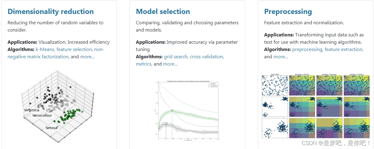
(1)機器學習庫(sklearn.linear_model)
代碼:
from sklearn import linear_model
from sklearn.linear_model import LinearRegression
import matplotlib.pyplot as plt#用於作圖
from pylab import *
mpl.rcParams['font.sans-serif'] = ['SimHei']
mpl.rcParams['axes.unicode_minus'] = False
import numpy as np#用於創建向量
reg=linear_model.LinearRegression(fit_intercept=True,normalize=False)
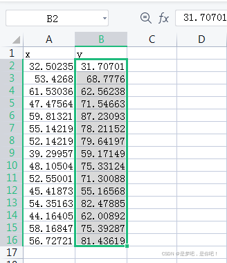
x=[[32.50235],[53.4268],[61.53036],[47.47564],[59.81321],[55.14219],[52.14219],[39.29957],
[48.10504],[52.55001],[45.41873],[54.35163],[44.16405],[58.16847],[56.72721]]
y=[31.70701,68.7776,62.56238,71.54663,87.23093,78.21152,79.64197,59.17149,75.33124,71.30088,55.16568,82.47885,62.00892
,75.39287,81.43619]
reg.fit(x,y)
k=reg.coef_#獲取斜率w1,w2,w3,...,wn
b=reg.intercept_#獲取截距w0
x0=np.arange(30,60,0.2)
y0=k*x0+b
print("k={0},b={1}".format(k,b))
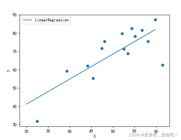
plt.scatter(x,y)
plt.plot(x0,y0,label='LinearRegression')
plt.xlabel('X')
plt.ylabel('Y')
plt.legend()
plt.show()
結果:
k=[1.36695374],b=0.13079331831460195
(2)Python詳細實現(方法1)
代碼:
#方法1
import numpy as np
import matplotlib.pyplot as plt
from pylab import *
mpl.rcParams['font.sans-serif'] = ['SimHei']
mpl.rcParams['axes.unicode_minus'] = False
#數據生成
data = []
for i in range(100):
    x = np.random.uniform(3., 12.)
    # mean=0, std=1
    eps = np.random.normal(0., 1)
    y = 1.677 * x + 0.039 + eps
    data.append([x, y])

data = np.array(data)

#統計誤差
# y = wx + b
def compute_error_for_line_given_points(b, w, points):
    totalError = 0
    for i in range(0, len(points)):
        x = points[i, 0]
        y = points[i, 1]
        # computer mean-squared-error
        totalError += (y - (w * x + b)) ** 2
    # average loss for each point
    return totalError / float(len(points))


#計算梯度
def step_gradient(b_current, w_current, points, learningRate):
    b_gradient = 0
    w_gradient = 0
    N = float(len(points))
    for i in range(0, len(points)):
        x = points[i, 0]
        y = points[i, 1]
        # grad_b = 2(wx+b-y)
        b_gradient += (2/N) * ((w_current * x + b_current) - y)
        # grad_w = 2(wx+b-y)*x
        w_gradient += (2/N) * x * ((w_current * x + b_current) - y)
    # update w'
    new_b = b_current - (learningRate * b_gradient)
    new_w = w_current - (learningRate * w_gradient)
    return [new_b, new_w]

#迭代更新
def gradient_descent_runner(points, starting_b, starting_w, learning_rate, num_iterations):
    b = starting_b
    w = starting_w
    # update for several times
    for i in range(num_iterations):
        b, w = step_gradient(b, w, np.array(points), learning_rate)
    return [b, w]


def main():

    learning_rate = 0.0001
    initial_b = 0  # initial y-intercept guess
    initial_w = 0  # initial slope guess
    num_iterations = 1000
    print("迭代前 b = {0}, w = {1}, error = {2}"
          .format(initial_b, initial_w,
                  compute_error_for_line_given_points(initial_b, initial_w, data))
          )
    print("Running...")
    [b, w] = gradient_descent_runner(data, initial_b, initial_w, learning_rate, num_iterations)
    print("第 {0} 次迭代結果 b = {1}, w = {2}, error = {3}".
          format(num_iterations, b, w,
                 compute_error_for_line_given_points(b, w, data))
          )
    plt.plot(data[:,0],data[:,1], color='b', marker='+', linestyle='--',label='true')
    plt.plot(data[:,0],w*data[:,0]+b,color='r',label='predict')
    plt.xlabel('X')
    plt.ylabel('Y')
    plt.legend()
    plt.show()


if __name__ == '__main__':
    main()
結果:
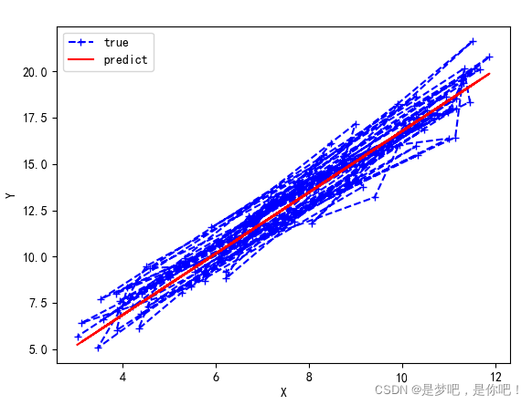
迭代前 :b = 0, w = 0, error = 186.61000821356697
Running…
第 1000 次迭代結果:b = 0.20558501549252192, w = 1.6589067569038516, error = 0.9963685680112963
(3)Python詳細實現(方法2)
代碼:
#方法2

import numpy as np
import pandas as pd
import matplotlib.pyplot as plt
import matplotlib as mpl
mpl.rcParams["font.sans-serif"]=["SimHei"]
mpl.rcParams["axes.unicode_minus"]=False


# y = wx + b
#Import data
file=pd.read_csv("data.csv")

def compute_error_for_line_given(b, w):
    totalError = np.sum((file['y']-(w*file['x']+b))**2)
    return np.mean(totalError)

def step_gradient(b_current, w_current,  learningRate):
    b_gradient = 0
    w_gradient = 0
    N = float(len(file['x']))
    for i in range (0,len(file['x'])):
        # grad_b = 2(wx+b-y)
        b_gradient += (2 / N) * ((w_current * file['x'] + b_current) - file['y'])
        # grad_w = 2(wx+b-y)*x
        w_gradient += (2 / N) * file['x'] * ((w_current * file['x'] + b_current) - file['x'])
    # update w'
    new_b = b_current - (learningRate * b_gradient)
    new_w = w_current - (learningRate * w_gradient)
    return [new_b, new_w]


def gradient_descent_runner( starting_b, starting_w, learning_rate, num_iterations):
    b = starting_b
    w = starting_w
    # update for several times
    for i in range(num_iterations):
        b, w = step_gradient(b, w,  learning_rate)
    return [b, w]


def main():
    learning_rate = 0.0001
    initial_b = 0  # initial y-intercept guess
    initial_w = 0  # initial slope guess
    num_iterations = 100
    print("Starting gradient descent at b = {0}, w = {1}, error = {2}"
          .format(initial_b, initial_w,
                  compute_error_for_line_given(initial_b, initial_w))
          )
    print("Running...")
    [b, w] = gradient_descent_runner(initial_b, initial_w, learning_rate, num_iterations)
    print("After {0} iterations b = {1}, w = {2}, error = {3}".
          format(num_iterations, b, w,
                 compute_error_for_line_given(b, w))
          )
    plt.plot(file['x'],file['y'],'ro',label='線性回歸')
    plt.xlabel('X')
    plt.ylabel('Y')
    plt.legend()
    plt.show()


if __name__ == '__main__':
    main()
結果:
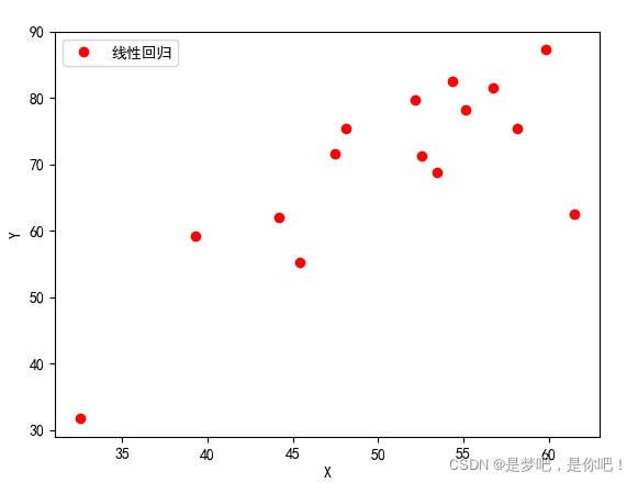
Starting gradient descent at b = 0, w = 0, error = 75104.71822821398
Running...
After 100 iterations b = 0     0.014845
1     0.325621
2     0.036883
3     0.502265
4     0.564917
5     0.479366
6     0.568968
7     0.422619
8     0.565073
9     0.393907
10    0.216854
11    0.580750
12    0.379350
13    0.361574
14    0.511651
dtype: float64, w = 0     0.999520
1     0.994006
2     0.999405
3     0.989645
4     0.990683
5     0.991444
6     0.989282
7     0.989573
8     0.988498
9     0.992633
10    0.995329
11    0.989490
12    0.991617
13    0.993872
14    0.991116
dtype: float64, error = 6451.5510231710905
數據:
(4)Python詳細實現(方法3)
#方法3

import numpy as np

points = np.genfromtxt("data.csv", delimiter=",")
#從數據讀入到返回需要兩個迭代循環,第一個迭代將文件中每一行轉化為一個字符串序列,
#第二個循環迭代對每個字符串序列指定合適的數據類型:
# y = wx + b
def compute_error_for_line_given_points(b, w, points):
    totalError = 0
    for i in range(0, len(points)):
        x = points[i, 0]
        y = points[i, 1]
        # computer mean-squared-error
        totalError += (y - (w * x + b)) ** 2
    # average loss for each point
    return totalError / float(len(points))


def step_gradient(b_current, w_current, points, learningRate):
    b_gradient = 0
    w_gradient = 0
    N = float(len(points))
    for i in range(0, len(points)):
        x = points[i, 0]
        y = points[i, 1]
        # grad_b = 2(wx+b-y)
        b_gradient += (2 / N) * ((w_current * x + b_current) - y)
        # grad_w = 2(wx+b-y)*x
        w_gradient += (2 / N) * x * ((w_current * x + b_current) - y)
    # update w'
    new_b = b_current - (learningRate * b_gradient)
    new_w = w_current - (learningRate * w_gradient)
    return [new_b, new_w]


def gradient_descent_runner(points, starting_b, starting_w, learning_rate, num_iterations):
    b = starting_b
    w = starting_w
    # update for several times
    for i in range(num_iterations):
        b, w = step_gradient(b, w, np.array(points), learning_rate)
    return [b, w]


def main():
    learning_rate = 0.0001
    initial_b = 0  # initial y-intercept guess
    initial_w = 0  # initial slope guess
    num_iterations = 1000
    print("Starting gradient descent at b = {0}, w = {1}, error = {2}"
          .format(initial_b, initial_w,
                  compute_error_for_line_given_points(initial_b, initial_w, points))
          )
    print("Running...")
    [b, w] = gradient_descent_runner(points, initial_b, initial_w, learning_rate, num_iterations)
    print("After {0} iterations b = {1}, w = {2}, error = {3}".
          format(num_iterations, b, w,
                 compute_error_for_line_given_points(b, w, points))
          )


if __name__ == '__main__':
    main()
4、案例——房屋與價格、尺寸

(1)代碼
#1.導入包
import matplotlib.pyplot as plt
import numpy as np
import pandas as pd
from sklearn import linear_model

#2.加載訓練數據,建立回歸方程
# 取數據集(1)
datasets_X = []     #存放房屋面積
datasets_Y = []     #存放交易價格
fr = open('房價與房屋尺寸.csv','r')    #讀取文件,r: 以隻讀方式打開文件,w: 打開一個文件隻用於寫入。
lines = fr.readlines()              #一次讀取整個文件。
for line in lines:                  #逐行進行操作,循環遍歷所有數據
    items = line.strip().split(',')    #去除數據文件中的逗號,strip()用於移除字符串頭尾指定的字符(默認為空格或換行符)或字符序列。
                                       #split(‘ '): 通過指定分隔符對字符串進行切片,如果參數 num 有指定值,則分隔 num+1 個子字符串。
    datasets_X.append(int(items[0]))   #將讀取的數據轉換為int型,並分別寫入
    datasets_Y.append(int(items[1]))

length = len(datasets_X)              #求得datasets_X的長度,即為數據的總數
datasets_X = np.array(datasets_X).reshape([length,1])   #將datasets_X轉化為數組,並變為1維,以符合線性回歸擬合函數輸入參數要求
datasets_Y = np.array(datasets_Y)                    #將datasets_Y轉化為數組

#取數據集(2)
'''fr = pd.read_csv('房價與房屋尺寸.csv',encoding='utf-8')
datasets_X=fr['房屋面積']
datasets_Y=fr['交易價格']'''

minX = min(datasets_X)
maxX = max(datasets_X)
X = np.arange(minX,maxX).reshape([-1,1])        #以數據datasets_X的最大值和最小值為范圍,建立等差數列,方便後續畫圖。
                                                #reshape([-1,1]),轉換成1列,reshape([2,-1]):轉換成兩行
linear = linear_model.LinearRegression()      #調用線性回歸模塊,建立回歸方程,擬合數據
linear.fit(datasets_X, datasets_Y)

#3.斜率及截距
print('Coefficients:', linear.coef_)      #查看回歸方程系數(k)
print('intercept:', linear.intercept_)    ##查看回歸方程截距(b)
print('y={0}x+{1}'.format(linear.coef_,linear.intercept_)) #擬合線

# 4.圖像中顯示
plt.scatter(datasets_X, datasets_Y, color = 'red')
plt.plot(X, linear.predict(X), color = 'blue')
plt.xlabel('Area')
plt.ylabel('Price')
plt.show()
(2)結果
Coefficients: [0.14198749]
intercept: 53.43633899175563
y=[0.14198749]x+53.43633899175563
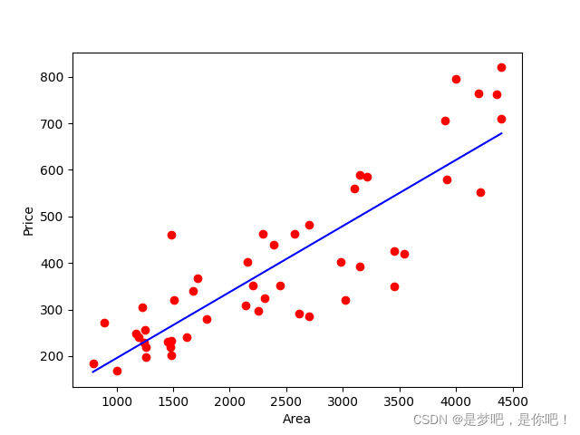
(3)數據
第一列是房屋面積,第二列是交易價格:
到此這篇關於人工智能—Python實現線性回歸的文章就介紹到這瞭,更多相關 Python實現線性回歸內容請搜索WalkonNet以前的文章或繼續瀏覽下面的相關文章希望大傢以後多多支持WalkonNet!