Python實現機器學習算法的分類
Python算法的分類
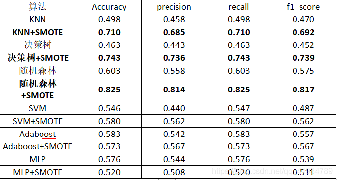
對葡萄酒數據集進行測試,由於數據集是多分類且數據的樣本分佈不平衡,所以直接對數據測試,效果不理想。所以使用SMOTE過采樣對數據進行處理,對數據去重,去空,處理後數據達到均衡,然後進行測試,與之前測試相比,準確率提升較高。
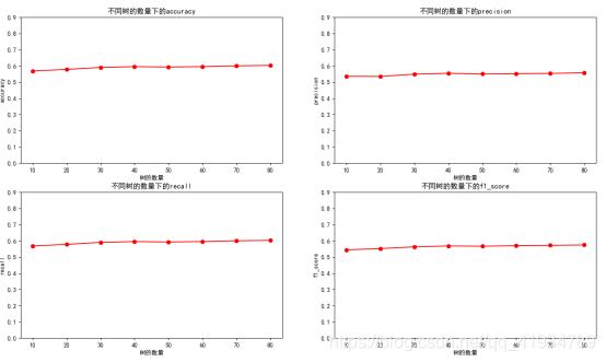
例如:決策樹:
Smote處理前:
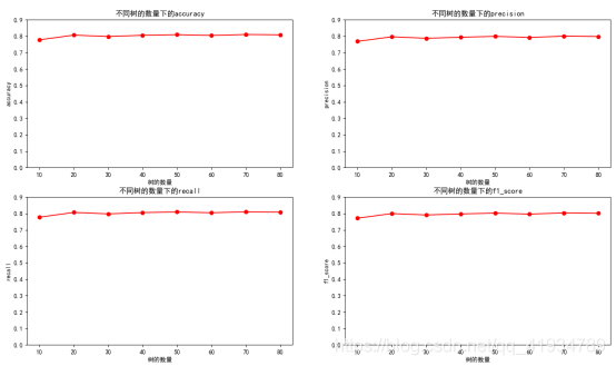
Smote處理後:
from typing import Counter
from matplotlib import colors, markers
import numpy as np
import pandas as pd
import operator
import matplotlib.pyplot as plt
from sklearn import tree
from sklearn.model_selection import train_test_split
from sklearn.ensemble import AdaBoostClassifier
from sklearn.ensemble import RandomForestClassifier
from sklearn.neighbors import KNeighborsClassifier
from sklearn.neural_network import MLPClassifier
from sklearn.svm import SVC
# 判斷模型預測準確率的模型
from sklearn.metrics import accuracy_score
from sklearn.metrics import roc_auc_score
from sklearn.metrics import f1_score
from sklearn.metrics import classification_report

#設置繪圖內的文字
plt.rcParams['font.family'] = ['sans-serif']
plt.rcParams['font.sans-serif'] = ['SimHei']


path ="C:\\Users\\zt\\Desktop\\winequality\\myexcel.xls"
# path=r"C:\\Users\\zt\\Desktop\\winequality\\winequality-red.csv"#您要讀取的文件路徑
# exceldata = np.loadtxt(
#     path,
#     dtype=str,
#     delimiter=";",#每列數據的隔開標志
#     skiprows=1
# )

# print(Counter(exceldata[:,-1]))

exceldata = pd.read_excel(path)
print(exceldata)

print(exceldata[exceldata.duplicated()])
print(exceldata.duplicated().sum())

#去重
exceldata = exceldata.drop_duplicates()


#判空去空
print(exceldata.isnull())
print(exceldata.isnull().sum)
print(exceldata[~exceldata.isnull()])
exceldata = exceldata[~exceldata.isnull()]

print(Counter(exceldata["quality"]))

#smote

#使用imlbearn庫中上采樣方法中的SMOTE接口
from imblearn.over_sampling import SMOTE
#定義SMOTE模型,random_state相當於隨機數種子的作用


X,y = np.split(exceldata,(11,),axis=1)
smo = SMOTE(random_state=10)

x_smo,y_smo = SMOTE().fit_resample(X.values,y.values)


print(Counter(y_smo))


x_smo = pd.DataFrame({"fixed acidity":x_smo[:,0], "volatile acidity":x_smo[:,1],"citric acid":x_smo[:,2] ,"residual sugar":x_smo[:,3] ,"chlorides":x_smo[:,4],"free sulfur dioxide":x_smo[:,5] ,"total sulfur dioxide":x_smo[:,6] ,"density":x_smo[:,7],"pH":x_smo[:,8] ,"sulphates":x_smo[:,9] ," alcohol":x_smo[:,10]})
y_smo = pd.DataFrame({"quality":y_smo})
print(x_smo.shape)
print(y_smo.shape)
#合並
exceldata = pd.concat([x_smo,y_smo],axis=1)
print(exceldata)

#分割X,y
X,y = np.split(exceldata,(11,),axis=1)
X_train,X_test,y_train,y_test = train_test_split(X,y,random_state=10,train_size=0.7)
print("訓練集大小:%d"%(X_train.shape[0]))
print("測試集大小:%d"%(X_test.shape[0]))


def func_mlp(X_train,X_test,y_train,y_test):
    print("神經網絡MLP:")
    kk = [i for i in range(200,500,50) ] #迭代次數
    t_precision = []
    t_recall = []
    t_accuracy = []
    t_f1_score = []
    for n in kk:
        method = MLPClassifier(activation="tanh",solver='lbfgs', alpha=1e-5,
                    hidden_layer_sizes=(5, 2), random_state=1,max_iter=n)
        method.fit(X_train,y_train)
        MLPClassifier(activation='relu', alpha=1e-05, batch_size='auto', beta_1=0.9,
                        beta_2=0.999, early_stopping=False, epsilon=1e-08,
                        hidden_layer_sizes=(5, 2), learning_rate='constant',
                        learning_rate_init=0.001, max_iter=n, momentum=0.9,
                        nesterovs_momentum=True, power_t=0.5, random_state=1, shuffle=True,
                        solver='lbfgs', tol=0.0001, validation_fraction=0.1, verbose=False,
                        warm_start=False)
        y_predict = method.predict(X_test)
        t =classification_report(y_test, y_predict, target_names=['3','4','5','6','7','8'],output_dict=True)
        print(t)
        t_accuracy.append(t["accuracy"])
        t_precision.append(t["weighted avg"]["precision"])
        t_recall.append(t["weighted avg"]["recall"])
        t_f1_score.append(t["weighted avg"]["f1-score"])
    plt.figure("數據未處理MLP")
    plt.subplot(2,2,1)
    #添加文本 #x軸文本
    plt.xlabel('迭代次數')
    #y軸文本
    plt.ylabel('accuracy')
    #標題
    plt.title('不同迭代次數下的accuracy')
    plt.plot(kk,t_accuracy,color="r",marker="o",lineStyle="-")
    plt.yticks(np.arange(0,1,0.1))

    plt.subplot(2,2,2)
    #添加文本 #x軸文本
    plt.xlabel('迭代次數')
    #y軸文本
    plt.ylabel('precision')
    #標題
    plt.title('不同迭代次數下的precision')
    plt.plot(kk,t_precision,color="r",marker="o",lineStyle="-")
    plt.yticks(np.arange(0,1,0.1))

    plt.subplot(2,2,3)
    #添加文本 #x軸文本
    plt.xlabel('迭代次數')
    #y軸文本
    plt.ylabel('recall')
    #標題
    plt.title('不同迭代次數下的recall')
    plt.plot(kk,t_recall,color="r",marker="o",lineStyle="-")
    plt.yticks(np.arange(0,1,0.1))

    plt.subplot(2,2,4)
    #添加文本 #x軸文本
    plt.xlabel('迭代次數')
    #y軸文本
    plt.ylabel('f1_score')
    #標題
    plt.title('不同迭代次數下的f1_score')
    plt.plot(kk,t_f1_score,color="r",marker="o",lineStyle="-")
    plt.yticks(np.arange(0,1,0.1))

    plt.show()


def func_svc(X_train,X_test,y_train,y_test):
    print("向量機:")
    kk = ["linear","poly","rbf"] #核函數類型
    t_precision = []
    t_recall = []
    t_accuracy = []
    t_f1_score = []
    for n in kk:
        method = SVC(kernel=n, random_state=0)
        method = method.fit(X_train, y_train)
        y_predic = method.predict(X_test)
        t =classification_report(y_test, y_predic, target_names=['3','4','5','6','7','8'],output_dict=True)
        print(t)
        t_accuracy.append(t["accuracy"])
        t_precision.append(t["weighted avg"]["precision"])
        t_recall.append(t["weighted avg"]["recall"])
        t_f1_score.append(t["weighted avg"]["f1-score"])
    plt.figure("數據未處理向量機")
    plt.subplot(2,2,1)
    #添加文本 #x軸文本
    plt.xlabel('核函數類型')
    #y軸文本
    plt.ylabel('accuracy')
    #標題
    plt.title('不同核函數類型下的accuracy')
    plt.plot(kk,t_accuracy,color="r",marker="o",lineStyle="-")
    plt.yticks(np.arange(0,1,0.1))

    plt.subplot(2,2,2)
    #添加文本 #x軸文本
    plt.xlabel('核函數類型')
    #y軸文本
    plt.ylabel('precision')
    #標題
    plt.title('不同核函數類型下的precision')
    plt.plot(kk,t_precision,color="r",marker="o",lineStyle="-")
    plt.yticks(np.arange(0,1,0.1))

    plt.subplot(2,2,3)
    #添加文本 #x軸文本
    plt.xlabel('核函數類型')
    #y軸文本
    plt.ylabel('recall')
    #標題
    plt.title('不同核函數類型下的recall')
    plt.plot(kk,t_recall,color="r",marker="o",lineStyle="-")
    plt.yticks(np.arange(0,1,0.1))

    plt.subplot(2,2,4)
    #添加文本 #x軸文本
    plt.xlabel('核函數類型')
    #y軸文本
    plt.ylabel('f1_score')
    #標題
    plt.title('不同核函數類型下的f1_score')
    plt.plot(kk,t_f1_score,color="r",marker="o",lineStyle="-")
    plt.yticks(np.arange(0,1,0.1))

    plt.show()

def func_classtree(X_train,X_test,y_train,y_test):
    print("決策樹:")
    kk = [10,20,30,40,50,60,70,80,90,100] #決策樹最大深度
    t_precision = []
    t_recall = []
    t_accuracy = []
    t_f1_score = []
    for n in kk:
        method = tree.DecisionTreeClassifier(criterion="gini",max_depth=n)
        method.fit(X_train,y_train)
        predic = method.predict(X_test)
        print("method.predict:%f"%method.score(X_test,y_test))


        t =classification_report(y_test, predic, target_names=['3','4','5','6','7','8'],output_dict=True)
        print(t)
        t_accuracy.append(t["accuracy"])
        t_precision.append(t["weighted avg"]["precision"])
        t_recall.append(t["weighted avg"]["recall"])
        t_f1_score.append(t["weighted avg"]["f1-score"])
    plt.figure("數據未處理決策樹")
    plt.subplot(2,2,1)
    #添加文本 #x軸文本
    plt.xlabel('決策樹最大深度')
    #y軸文本
    plt.ylabel('accuracy')
    #標題
    plt.title('不同決策樹最大深度下的accuracy')
    plt.plot(kk,t_accuracy,color="r",marker="o",lineStyle="-")
    plt.yticks(np.arange(0,1,0.1))

    plt.subplot(2,2,2)
    #添加文本 #x軸文本
    plt.xlabel('決策樹最大深度')
    #y軸文本
    plt.ylabel('precision')
    #標題
    plt.title('不同決策樹最大深度下的precision')
    plt.plot(kk,t_precision,color="r",marker="o",lineStyle="-")
    plt.yticks(np.arange(0,1,0.1))

    plt.subplot(2,2,3)
    #添加文本 #x軸文本
    plt.xlabel('決策樹最大深度')
    #y軸文本
    plt.ylabel('recall')
    #標題
    plt.title('不同決策樹最大深度下的recall')
    plt.plot(kk,t_recall,color="r",marker="o",lineStyle="-")
    plt.yticks(np.arange(0,1,0.1))

    plt.subplot(2,2,4)
    #添加文本 #x軸文本
    plt.xlabel('決策樹最大深度')
    #y軸文本
    plt.ylabel('f1_score')
    #標題
    plt.title('不同決策樹最大深度下的f1_score')
    plt.plot(kk,t_f1_score,color="r",marker="o",lineStyle="-")
    plt.yticks(np.arange(0,1,0.1))

    plt.show()

def func_adaboost(X_train,X_test,y_train,y_test):
    print("提升樹:")
    kk = [0.1,0.2,0.3,0.4,0.5,0.6,0.7,0.8]
    t_precision = []
    t_recall = []
    t_accuracy = []
    t_f1_score = []
    for n in range(100,200,200):
        for k in kk:
            print("迭代次數為:%d\n學習率:%.2f"%(n,k))
            bdt = AdaBoostClassifier(tree.DecisionTreeClassifier(max_depth=2, min_samples_split=20),
                                    algorithm="SAMME",
                                    n_estimators=n, learning_rate=k)
            bdt.fit(X_train, y_train)
            #迭代100次 ,學習率為0.1
            y_pred = bdt.predict(X_test)
            print("訓練集score:%lf"%(bdt.score(X_train,y_train)))
            print("測試集score:%lf"%(bdt.score(X_test,y_test)))
            print(bdt.feature_importances_)

            t =classification_report(y_test, y_pred, target_names=['3','4','5','6','7','8'],output_dict=True)
            print(t)
            t_accuracy.append(t["accuracy"])
            t_precision.append(t["weighted avg"]["precision"])
            t_recall.append(t["weighted avg"]["recall"])
            t_f1_score.append(t["weighted avg"]["f1-score"])
    plt.figure("數據未處理迭代100次(adaboost)")
    plt.subplot(2,2,1)
    #添加文本 #x軸文本
    plt.xlabel('學習率')
    #y軸文本
    plt.ylabel('accuracy')
    #標題
    plt.title('不同學習率下的accuracy')
    plt.plot(kk,t_accuracy,color="r",marker="o",lineStyle="-")
    plt.yticks(np.arange(0,1,0.1))

    plt.subplot(2,2,2)
    #添加文本 #x軸文本
    plt.xlabel('學習率')
    #y軸文本
    plt.ylabel('precision')
    #標題
    plt.title('不同學習率下的precision')
    plt.plot(kk,t_precision,color="r",marker="o",lineStyle="-")
    plt.yticks(np.arange(0,1,0.1))

    plt.subplot(2,2,3)
    #添加文本 #x軸文本
    plt.xlabel('學習率')
    #y軸文本
    plt.ylabel('recall')
    #標題
    plt.title('不同學習率下的recall')
    plt.plot(kk,t_recall,color="r",marker="o",lineStyle="-")
    plt.yticks(np.arange(0,1,0.1))

    plt.subplot(2,2,4)
    #添加文本 #x軸文本
    plt.xlabel('學習率')
    #y軸文本
    plt.ylabel('f1_score')
    #標題
    plt.title('不同學習率下的f1_score')
    plt.plot(kk,t_f1_score,color="r",marker="o",lineStyle="-")
    plt.yticks(np.arange(0,1,0.1))

    plt.show()


# inX 用於分類的輸入向量
# dataSet表示訓練樣本集
# 標簽向量為labels,標簽向量的元素數目和矩陣dataSet的行數相同
# 參數k表示選擇最近鄰居的數目
def classify0(inx, data_set, labels, k):
    """實現k近鄰"""
    data_set_size = data_set.shape[0]   # 數據集個數,即行數
    diff_mat = np.tile(inx, (data_set_size, 1)) - data_set   # 各個屬性特征做差
    sq_diff_mat = diff_mat**2  # 各個差值求平方
    sq_distances = sq_diff_mat.sum(axis=1)  # 按行求和
    distances = sq_distances**0.5   # 開方
    sorted_dist_indicies = distances.argsort()  # 按照從小到大排序,並輸出相應的索引值
    class_count = {}  # 創建一個字典,存儲k個距離中的不同標簽的數量

    for i in range(k):
        vote_label = labels[sorted_dist_indicies[i]]  # 求出第i個標簽

        # 訪問字典中值為vote_label標簽的數值再加1,
        #class_count.get(vote_label, 0)中的0表示當為查詢到vote_label時的默認值
        class_count[vote_label[0]] = class_count.get(vote_label[0], 0) + 1
    # 將獲取的k個近鄰的標簽類進行排序
    sorted_class_count = sorted(class_count.items(),
    key=operator.itemgetter(1), reverse=True)
    # 標簽類最多的就是未知數據的類
    return sorted_class_count[0][0]

def func_knn(X_train,X_test,y_train,y_test):
    print("k近鄰:")
    kk = [i for i in range(3,30,5)] #k的取值
    t_precision = []
    t_recall = []
    t_accuracy = []
    t_f1_score = []
    for n in kk:
        y_predict = []
        for x in X_test.values:
            a = classify0(x, X_train.values, y_train.values, n)  # 調用k近鄰分類
            y_predict.append(a)

        t =classification_report(y_test, y_predict, target_names=['3','4','5','6','7','8'],output_dict=True)
        print(t)
        t_accuracy.append(t["accuracy"])
        t_precision.append(t["weighted avg"]["precision"])
        t_recall.append(t["weighted avg"]["recall"])
        t_f1_score.append(t["weighted avg"]["f1-score"])
    plt.figure("數據未處理k近鄰")
    plt.subplot(2,2,1)
    #添加文本 #x軸文本
    plt.xlabel('k值')
    #y軸文本
    plt.ylabel('accuracy')
    #標題
    plt.title('不同k值下的accuracy')
    plt.plot(kk,t_accuracy,color="r",marker="o",lineStyle="-")
    plt.yticks(np.arange(0,1,0.1))

    plt.subplot(2,2,2)
    #添加文本 #x軸文本
    plt.xlabel('k值')
    #y軸文本
    plt.ylabel('precision')
    #標題
    plt.title('不同k值下的precision')
    plt.plot(kk,t_precision,color="r",marker="o",lineStyle="-")
    plt.yticks(np.arange(0,1,0.1))

    plt.subplot(2,2,3)
    #添加文本 #x軸文本
    plt.xlabel('k值')
    #y軸文本
    plt.ylabel('recall')
    #標題
    plt.title('不同k值下的recall')
    plt.plot(kk,t_recall,color="r",marker="o",lineStyle="-")
    plt.yticks(np.arange(0,1,0.1))

    plt.subplot(2,2,4)
    #添加文本 #x軸文本
    plt.xlabel('k值')
    #y軸文本
    plt.ylabel('f1_score')
    #標題
    plt.title('不同k值下的f1_score')
    plt.plot(kk,t_f1_score,color="r",marker="o",lineStyle="-")
    plt.yticks(np.arange(0,1,0.1))

    plt.show()

def func_randomforest(X_train,X_test,y_train,y_test):
    print("隨機森林:")
    t_precision = []
    t_recall = []
    t_accuracy = []
    t_f1_score = []
    kk = [10,20,30,40,50,60,70,80] #默認樹的數量
    for n in kk:
        clf = RandomForestClassifier(n_estimators=n, max_depth=100,min_samples_split=2, random_state=10,verbose=True)
        clf.fit(X_train,y_train)
        predic = clf.predict(X_test)

        print("特征重要性:",clf.feature_importances_)
        print("acc:",clf.score(X_test,y_test))

        t =classification_report(y_test, predic, target_names=['3','4','5','6','7','8'],output_dict=True)
        print(t)
        t_accuracy.append(t["accuracy"])
        t_precision.append(t["weighted avg"]["precision"])
        t_recall.append(t["weighted avg"]["recall"])
        t_f1_score.append(t["weighted avg"]["f1-score"])
    plt.figure("數據未處理深度100(隨機森林)")
    plt.subplot(2,2,1)
    #添加文本 #x軸文本
    plt.xlabel('樹的數量')
    #y軸文本
    plt.ylabel('accuracy')
    #標題
    plt.title('不同樹的數量下的accuracy')
    plt.plot(kk,t_accuracy,color="r",marker="o",lineStyle="-")
    plt.yticks(np.arange(0,1,0.1))

    plt.subplot(2,2,2)
    #添加文本 #x軸文本
    plt.xlabel('樹的數量')
    #y軸文本
    plt.ylabel('precision')
    #標題
    plt.title('不同樹的數量下的precision')
    plt.plot(kk,t_precision,color="r",marker="o",lineStyle="-")
    plt.yticks(np.arange(0,1,0.1))

    plt.subplot(2,2,3)
    #添加文本 #x軸文本
    plt.xlabel('樹的數量')
    #y軸文本
    plt.ylabel('recall')
    #標題
    plt.title('不同樹的數量下的recall')
    plt.plot(kk,t_recall,color="r",marker="o",lineStyle="-")
    plt.yticks(np.arange(0,1,0.1))

    plt.subplot(2,2,4)
    #添加文本 #x軸文本
    plt.xlabel('樹的數量')
    #y軸文本
    plt.ylabel('f1_score')
    #標題
    plt.title('不同樹的數量下的f1_score')
    plt.plot(kk,t_f1_score,color="r",marker="o",lineStyle="-")
    plt.yticks(np.arange(0,1,0.1))

    plt.show()


if __name__ == '__main__':
    #神經網絡
    print(func_mlp(X_train,X_test,y_train,y_test))
    #向量機
    print(func_svc(X_train,X_test,y_train,y_test))
    #決策樹
    print(func_classtree(X_train,X_test,y_train,y_test))
    #提升樹
    print(func_adaboost(X_train,X_test,y_train,y_test))
    #knn
    print(func_knn(X_train,X_test,y_train,y_test))
    #randomforest
    print(func_randomforest(X_train,X_test,y_train,y_test))
到此這篇關於Python實現機器學習算法的分類的文章就介紹到這瞭,更多相關Python算法分類內容請搜索WalkonNet以前的文章或繼續瀏覽下面的相關文章希望大傢以後多多支持WalkonNet!
推薦閱讀:
- Python利用Seaborn繪制多標簽的混淆矩陣
- Python數據分析應用之Matplotlib數據可視化詳情
- 使用Python處理KNN分類算法的實現代碼
- python數據可視化plt庫實例詳解
- 基於numpy實現邏輯回歸