Python機器學習應用之基於天氣數據集的XGBoost分類篇解讀
一、XGBoost
XGBoost並不是一種模型,而是一個可供用戶輕松解決分類、回歸或排序問題的軟件包。
1 XGBoost的優點
- 簡單易用。相對其他機器學習庫,用戶可以輕松使用XGBoost並獲得相當不錯的效果。
- 高效可擴展。在處理大規模數據集時速度快效果好,對內存等硬件資源要求不高。
- 魯棒性強。相對於深度學習模型不需要精細調參便能取得接近的效果。
- XGBoost內部實現提升樹模型,可以自動處理缺失值。
2 XGBoost的缺點
- 相對於深度學習模型無法對時空位置建模,不能很好地捕獲圖像、語音、文本等高維數據。
- 在擁有海量訓練數據,並能找到合適的深度學習模型時,深度學習的精度可以遙遙領先XGBoost。
二、實現過程
1 數據集
天氣數據集 提取碼:1234
2 實現
#%%導入基本庫
import numpy as np
import pandas as pd

## 繪圖函數庫
import matplotlib.pyplot as plt
import seaborn as sns
#讀取數據
data=pd.read_csv('D:\Python\ML\data\XGBtrain.csv')
通過variable explorer查看樣本數據

也可以使用head()或tail()函數,查看樣本前幾行和後幾行。不難看出,數據集中含有NAN,代表數據中存在缺失值,可能是在數據采集或者處理過程中產生的一種錯誤,此處采用-1將缺失值進行填充,還有其他的填充方法:
- 中位數填補
- 平均數填補
註:在數據的前期處理中,一定要註意對缺失值的處理。前期數據處理的結果將會嚴重影響後面是否可能得到合理的結果
data=data.fillna(-1)
#利用value_counts()函數查看訓練集標簽的數量(Raintomorrow=no)
print(pd.Series(data['RainTomorrow']).value_counts())
data_des=data.describe()
填充後:

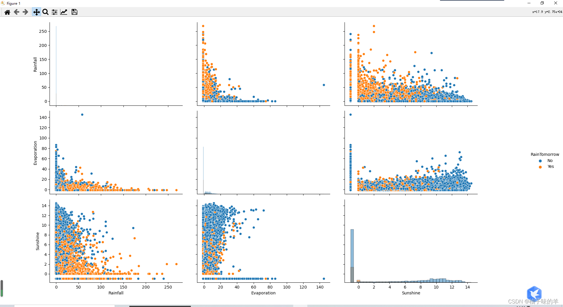
#%%#可視化數據(特征值包括數字特征和非數字特征)
numerical_features = [x for x in data.columns if data[x].dtype == np.float]
category_features = [x for x in data.columns if data[x].dtype != np.float and x != 'RainTomorrow']
#%% 選取三個特征與標簽組合的散點可視化
sns.pairplot(data=data[['Rainfall','Evaporation','Sunshine'] + ['RainTomorrow']], diag_kind='hist', hue= 'RainTomorrow')
plt.show()
#%%每個特征的箱圖
i=0
for col in data[numerical_features].columns:
    if col != 'RainTomorrow':
        plt.subplot(2,8,i+1)
        sns.boxplot(x='RainTomorrow', y=col, saturation=0.5, palette='pastel', data=data)
        plt.title(col)
        i=i+1
plt.show()

#%%非數字特征
tlog = {}
for i in category_features:
    tlog[i] = data[data['RainTomorrow'] == 'Yes'][i].value_counts()
flog = {}
for i in category_features:
    flog[i] = data[data['RainTomorrow'] == 'No'][i].value_counts()
#%%不同地區下雨情況
plt.figure(figsize=(20,10))
plt.subplot(1,2,1)
plt.title('RainTomorrow')
sns.barplot(x = pd.DataFrame(tlog['Location']).sort_index()['Location'], y = pd.DataFrame(tlog['Location']).sort_index().index, color = "red")
plt.subplot(1,2,2)
plt.title('Not RainTomorrow')
sns.barplot(x = pd.DataFrame(flog['Location']).sort_index()['Location'], y = pd.DataFrame(flog['Location']).sort_index().index, color = "blue")
plt.show()

#%%
plt.figure(figsize=(20,5))
plt.subplot(1,2,1)
plt.title('RainTomorrow')
sns.barplot(x = pd.DataFrame(tlog['RainToday'][:2]).sort_index()['RainToday'], y = pd.DataFrame(tlog['RainToday'][:2]).sort_index().index, color = "red")
plt.subplot(1,2,2)
plt.title('Not RainTomorrow')
sns.barplot(x = pd.DataFrame(flog['RainToday'][:2]).sort_index()['RainToday'], y = pd.DataFrame(flog['RainToday'][:2]).sort_index().index, color = "blue")
plt.show()

XGBoost無法處理字符串類型的數據,需要將字符串數據轉化成數值
#%%對離散變量進行編碼
## 把所有的相同類別的特征編碼為同一個值
def get_mapfunction(x):
mapp = dict(zip(x.unique().tolist(),
range(len(x.unique().tolist()))))
def mapfunction(y):
if y in mapp:
return mapp[y]
else:
return -1
return mapfunction
#將非數字特征離散化
for i in category_features:
data[i] = data[i].apply(get_mapfunction(data[i]))
#%%利用XGBoost進行訓練與預測
## 為瞭正確評估模型性能,將數據劃分為訓練集和測試集,並在訓練集上訓練模型,在測試集上驗證模型性能。
from sklearn.model_selection import train_test_split
## 選擇其類別為0和1的樣本 (不包括類別為2的樣本)
data_target_part = data['RainTomorrow']
data_features_part = data[[x for x in data.columns if x != 'RainTomorrow']]
## 測試集大小為20%, 80%/20%分
x_train, x_test, y_train, y_test = train_test_split(data_features_part, data_target_part, test_size = 0.2, random_state = 2020)
#%%導入XGBoost模型
from xgboost.sklearn import XGBClassifier
## 定義 XGBoost模型
clf = XGBClassifier()
# 在訓練集上訓練XGBoost模型
clf.fit(x_train, y_train)
#%% 在訓練集和測試集上分佈利用訓練好的模型進行預測
train_predict = clf.predict(x_train)
test_predict = clf.predict(x_test)
from sklearn import metrics
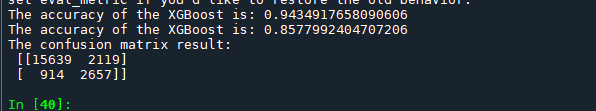
## 利用accuracy(準確度)【預測正確的樣本數目占總預測樣本數目的比例】評估模型效果
print('The accuracy of the XGBoost is:',metrics.accuracy_score(y_train,train_predict))
print('The accuracy of the XGBoost is:',metrics.accuracy_score(y_test,test_predict))
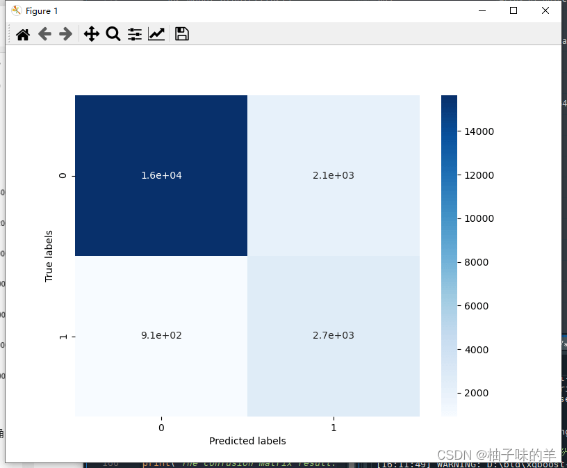
## 查看混淆矩陣 (預測值和真實值的各類情況統計矩陣)
confusion_matrix_result = metrics.confusion_matrix(test_predict,y_test)
print('The confusion matrix result:\n',confusion_matrix_result)
# 利用熱力圖對於結果進行可視化
plt.figure(figsize=(8, 6))
sns.heatmap(confusion_matrix_result, annot=True, cmap='Blues')
plt.xlabel('Predicted labels')
plt.ylabel('True labels')
plt.show()

#%%利用XGBoost進行特征選擇:
#XGboost中可以用屬性feature_importances_去查看特征的重要度。
sns.barplot(y=data_features_part.columns,x=clf.feature_importances_)

初次之外,我們還可以使用XGBoost中的下列重要屬性來評估特征的重要性:
- weight:是以特征用到的次數來評價
- gain:當利用特征做劃分的時候的評價基尼指數
- cover:利用一個覆蓋樣本的指標二階導數(具體原理不清楚有待探究)平均值來劃分。
- total_gain:總基尼指數
- total_cover:總覆蓋
#利用XGBoost的其他重要參數評估特征的重要性
from sklearn.metrics import accuracy_score
from xgboost import plot_importance

def estimate(model,data):
    #sns.barplot(data.columns,model.feature_importances_)
    ax1=plot_importance(model,importance_type="gain")
    ax1.set_title('gain')
    ax2=plot_importance(model, importance_type="weight")
    ax2.set_title('weight')
    ax3 = plot_importance(model, importance_type="cover")
    ax3.set_title('cover')
    plt.show()
def classes(data,label,test):
    model=XGBClassifier()
    model.fit(data,label)
    ans=model.predict(test)
    estimate(model, data)
    return ans

ans=classes(x_train,y_train,x_test)
pre=accuracy_score(y_test, ans)
print('acc=',accuracy_score(y_test,ans))


XGBoost中包括但不限於下列對模型影響較大的參數:
- learning_rate: 有時也叫作eta,系統默認值為0.3。每一步迭代的步長,很重要。太大瞭運行準確率不高,太小瞭運行速度慢。
- subsample:系統默認為1。這個參數控制對於每棵樹,隨機采樣的比例。減小這個參數的值,算法會更加保守,避免過擬合, 取值范圍零到一。
- colsample_bytree:系統默認值為1。我們一般設置成0.8左右。用來控制每棵隨機采樣的列數的占比(每一列是一個特征)。max_depth: 系統默認值為6,我們常用3-10之間的數字。這個值為樹的最大深度。這個值是用來控制過擬合的。
- max_depth越大,模型學習的更加具體。
調節模型參數的方法有貪心算法、網格調參、貝葉斯調參等。這裡我們采用網格調參,它的基本思想是窮舉搜索:在所有候選的參數選擇中,通過循環遍歷,嘗試每一種可能性,表現最好的參數就是最終的結果
#%%通過調參獲得更好的效果
## 從sklearn庫中導入網格調參函數
from sklearn.model_selection import GridSearchCV

## 定義參數取值范圍
learning_rate = [0.1, 0.3, 0.6]
subsample = [0.8, 0.9]
colsample_bytree = [0.6, 0.8]
max_depth = [3,5,8]

parameters = { 'learning_rate': learning_rate,
              'subsample': subsample,
              'colsample_bytree':colsample_bytree,
              'max_depth': max_depth}
model = XGBClassifier(n_estimators = 50)

## 進行網格搜索
clf = GridSearchCV(model, parameters, cv=3, scoring='accuracy',verbose=1,n_jobs=-1)
clf = clf.fit(x_train, y_train)
#%%網格搜索後的參數
print(clf.best_params_)

#%% 在訓練集和測試集上分別利用最好的模型參數進行預測
## 定義帶參數的 XGBoost模型
clf = XGBClassifier(colsample_bytree = 0.6, learning_rate = 0.3, max_depth= 8, subsample = 0.9)
# 在訓練集上訓練XGBoost模型
clf.fit(x_train, y_train)

train_predict = clf.predict(x_train)
test_predict = clf.predict(x_test)

## 利用accuracy(準確度)【預測正確的樣本數目占總預測樣本數目的比例】評估模型效果
print('The accuracy of the Logistic Regression is:',metrics.accuracy_score(y_train,train_predict))
print('The accuracy of the Logistic Regression is:',metrics.accuracy_score(y_test,test_predict))

## 查看混淆矩陣 (預測值和真實值的各類情況統計矩陣)
confusion_matrix_result = metrics.confusion_matrix(test_predict,y_test)
print('The confusion matrix result:\n',confusion_matrix_result)

# 利用熱力圖對於結果進行可視化
plt.figure(figsize=(8, 6))
sns.heatmap(confusion_matrix_result, annot=True, cmap='Blues')
plt.xlabel('Predicted labels')
plt.ylabel('True labels')
plt.show()
三、Keys
XGBoost的重要參數
- eta【默認0.3】:通過為每一顆樹增加權重,提高模型的魯棒性。典型值為0.01-0.2。
- min_child_weight【默認1】:決定最小葉子節點樣本權重和。這個參數可以避免過擬合。當它的值較大時,可以避免模型學習到局部的特殊樣本。但是如果這個值過高,則會導致模型擬合不充分。
- max_depth【默認6】:這個值也是用來避免過擬合的,max_depth越大,模型會學到更具體更局部的樣本。典型值:3-10
- max_leaf_nodes:樹上最大的節點或葉子的數量。可以替代max_depth的作用。這個參數的定義會導致忽略max_depth參數。
- gamma【默認0】:在節點分裂時,隻有分裂後損失函數的值下降瞭,才會分裂這個節點。Gamma指定瞭節點分裂所需的最小損失函數下降值。這個參數的值越大,算法越保守。這個參數的值和損失函數息息相關。
- max_delta_step【默認0】:這個參數限制每棵樹權重改變的最大步長。如果這個參數的值為0,那就意味著沒有約束。如果它被賦予瞭某個正值,那麼它會讓這個算法更加保守。但是當各類別的樣本十分不平衡時,它對分類問題是很有幫助的。
- subsample【默認1】:這個參數控制對於每棵樹,隨機采樣的比例。減小這個參數的值,算法會更加保守,避免過擬合。但是,如果這個值設置得過小,它可能會導致欠擬合。典型值:0.5-1
- colsample_bytree【默認1】:用來控制每棵隨機采樣的列數的占比(每一列是一個特征)。典型值:0.5-1
- colsample_bylevel【默認1】:用來控制樹的每一級的每一次分裂,對列數的采樣的占比。subsample參數和colsample_bytree參數可以起到相同的作用,一般用不到。
- lambda【默認1】:權重的L2正則化項。(和Ridge regression類似)。這個參數是用來控制XGBoost的正則化部分的。雖然大部分數據科學傢很少用到這個參數,但是這個參數在減少過擬合上還是可以挖掘出更多用處的。
- alpha【默認1】:權重的L1正則化項。(和Lasso regression類似)。可以應用在很高維度的情況下,使得算法的速度更快。
- scale_pos_weight【默認1】:在各類別樣本十分不平衡時,把這個參數設定為一個正值,可以使算法更快收斂。
886~~
到此這篇關於Python機器學習應用之基於天氣數據集的XGBoost分類篇解讀的文章就介紹到這瞭,更多相關Python XGBoost內容請搜索WalkonNet以前的文章或繼續瀏覽下面的相關文章希望大傢以後多多支持WalkonNet!
推薦閱讀:
- Python機器學習應用之決策樹分類實例詳解
- Python機器學習應用之基於LightGBM的分類預測篇解讀
- Python機器學習應用之基於BP神經網絡的預測篇詳解
- Python集成學習之Blending算法詳解
- python生成器generator:深度學習讀取batch圖片的操作